Ergodicity: the Most Over-Looked Assumption

Consider two ways of making purple.

Method 1: Alternate red and blue squares. With enough squares, purple emerges.

Method 2: Make square alternate between red and blue. With short enough time intervals, purple emerges.

First method made changes in the space (ensemble) dimension.

Second method made changes in the time (temporal) dimension.

Both converged to give the same result (purple). This is ergodicity.

A process is said to be ergodic if the ensemble-average is equal to the time-average.

This simple idea has ground-breaking implications in physics, finance, economics, physics, and even everyday life.

Ergodicity is surprisingly prevalent in a vast multitude of systems.

Much like Black Swans, antifragility, non-linearity, and optionality, it’s another concept that Nassim Taleb has raised his voice on. But this one has garnered far less attention than others.

The problem is, ergodicity is generally poorly understood.

Making matters worse, every article or video I’ve found on this tends to over-complicate it.

And hence I write this post:

1. Going bust despite favourable odds: A gambling example illustrating ergodicity and the Kelly criterion
2. Ergodocity economics: Prevalence and dangers of the ergodic assumption in modern portfolio theory, DCF models, and GDP
3. Living in bets: How I’m personally applying ergodicity concepts to life

 

---

1. Going bust despite favourable odds

1.1. Definition

A process is said to be ergodic if the ensemble-average and time-average is equivalent.

A more formal definition from Ole Peters from his Dec-19 Nature journal article:

The ergodic hypothesis is a key analytical device of equilibrium statistical mechanics. It underlies the assumption that the time average and the expectation value of an observable are the same. Where it is valid, dynamical descriptions can often be replaced with much simpler probabilistic ones — time is essentially eliminated from the models.

A mouthful right?

Let’s park the definition here for now, and take baby steps with a more digestible example.

 

1.2. Rigged coin flip game

Flip a coin. If heads, your net wealth is increased by 50%. If tails, your net wealth is decreased by 40%.

Would you play? If so, how many times?

At first glance it seems like the game is rigged in your favour. We expect an equal number of heads and tails in the long run. Given you are paid more from each head than you are penalised for on each tail, you should just play as many times as possible right? Besides, even if you end up on a losing streak, you don’t ever lose all your money, you only lose 40% of whatever you were on. You can win it back with the favourable payoffs. Right?

Well, here’s a simulation of what could happen if you played 50 times.

• Horizontal axis is time.
• Vertical axis is net worth, a function of time.
• N=1 means we’re looking at the outcome for 1 individual.

There doesn’t seem to be a trend here. We were expecting an upward gradient given the favourable odds. But we end up at a loss. Strange. Maybe this guy was unlucky?

Let’s extend the simulation for this one individual into 1,000 rounds.

Looks like they’re stuck at zero. This is surprisingly given the favourable odds. We expected the math to offset the unlucky first 50 rounds. Is this guy just really unlucky? 

Well here’s the same chart as above but with a logarithmic axis. 

Remember they never go completely bust – since a loss is 40% of their current wealth. Now, the downward trend is rather apparent.

Back to our first graph.

This was a simulation for 1 individual over 50 rounds.

Now, let’s run simulations for 100 individuals playing concurrently over 50 rounds, and show the average results (wealth) at each point in time in one image.

The green line shows the average y-values (wealth) for 100 players at each x-value (time). Again, no clear trend.

Simulate for 10,000 players (red line) and we start to see a trend. On average, this group of 10,000 players is sitting on a nice ~10x profit.

Simulate a million concurrent players, and the trend is more apparent. 

Again, a logarithmic axis shows this more clearly.

The average wealth of a million people increases exponentially as they play this game. (Note: linear increase on logarithmic axis means exponential growth. It’s a neat trick to distinguish exponential growth from mere very fast growth.)

This trend persists as we extend time to 1,000 rounds and so on. 

 

But wait. This doesn’t make sense.

Earlier, we showed that for an individual player, wealth trends to zero over time.

But for the aggregate of individuals, wealth trends exponentially upwards over time.

How can many things that trend to zero sum up to exponential growth?

Answer: there’s a few really lucky bastards that distort the average.

A more technical answer: ergodicity. Or more specifically, a false assumption of ergodicity for this non-ergodic game.

 

Let’s take a deeper dive and explore some scenarios for an individual starting with $100.

Round 1: 2 scenarios

• H: $100 x 1.5 = $150 (up $50)
• T: $100 x 0.6 = $60 (down $40)
• Outcomes: 1 up, 1 down 50% of outcomes are up.
• Average after 1 round: $105

Round 2: 4 scenarios

• HH: $100 x 1.5 x 1.5 = $225 (up $125)
• HT: $100 x 1.5 x 0.6 = $90 (down $10)
• TH: $100 x 0.6 x 1.5 = $90 (down $10)
• TT: $100 x 0.6 x 0.6 = $36 (down $64)
• Outcomes: 1 up, 3 down. 25% of outcomes are up.
• Average after 2 rounds: $110.3

Round 3: 8 scenarios

• HHH: $100 x 1.5 x 1.5 x 1.5  = $337.5 (up $237.5)
• HTH: $100 x 1.5 x 0.6 x 1.5 = $135 (up $35)
• THH: $100 x 0.6 x 1.5 x 1.5 = $135 (up $35)
• TTH: $100 x 0.6 x 0.6 x 1.5 = $54 (down $66)
• HHT: $100 x 1.5 x 1.5 x 0.6 = $135 (up $35)
• HTT: $100 x 1.5 x 0.6 x 0.6 = $54 (down $66)
• THT: $100 x 0.6 x 1.5 x 0.6 = $54 (down $66)
• TTT: $100 x 0.6 x 0.6 x 0.6 = $21.6 (down $78.4)
• Outcomes: 4 up, 4 down. 50% of outcomes are up.
• Average after 3 rounds: $115.8

Similarly, we repeat this logic for even more rounds with the help of binomial probability distributions in Excel.

Round 10: 1,024 scenarios

• H 10 times: $100 x 1.5¹⁰ = $5,767
• H 5 times, T 5 times (order doesn’t matter here): $100 x 1.5⁵ x 0.6⁵ = $59
• T 10 times: $100 x 0.6¹⁰ = $0.6
• Outcomes: 386 up, 638 down. 38% of outcomes are up..
• Average after 10 rounds: $163 ($100 x 1.05¹⁰).

Round 100: 2¹⁰⁰ scenarios

• H 100 times: $100 x 1.5¹⁰⁰ = $4.1 x 10¹⁹
• H 50 times, T 50 times (order doesn’t matter here): $100 x 1.5⁵⁰ x 0.6⁵ = $0.5
• T 100 times: $100 x 0.6¹⁰⁰ = $6.5 x 10^-21
• Outcomes: 1.7 x 10²⁹ up, 1.1 x 10³⁰ down. 14% of outcomes are up.
• Average after 100 rounds: $13,150 ($100 x 1.05¹⁰⁰)

Some observations.

(i) In aggregate, payout is favourable to the players since average wealth is consistently above starting value of $100. This is the ensemble-average.

(ii) But this asymmetric payoff is only favourable on the ensemble dimension (taking the aggregate and dividing it by number of players). The pay-off structure is not favourable to an individual on the temporal (time) dimension. On an individual level, people are actually more likely to lose the longer they play. Gambler’s ruin. Thus, looking at ensemble returns is a poor indicator of individual returns.

So as the game goes on: the house loses money as they’re paying out more than they receive, while more people become losers, and just a lucky few get obscenely rich. (For context, the winnings from 100 consecutive heads, $4.1 x 10¹⁹ is taking the global GDP of ~$100t and multiplying it by 400k years. So all of the wealth we’re creating today multiplied by longer than Homo sapiens’ existence. The probability of 1 in 2¹⁰⁰ is even more ludicrous.)

There’s many variations to the example we explored: e.g. a triple-or-nothing coin flip. We get similar results except instead of decaying to zero, people go completely bust and end the game there, while some extremely lucky get fanatically rich.

 

1.3. Back to ergodicity

Recall:

A process is said to be ergodic if the ensemble-average and time-average are equivalent.

Clearly, simulating an individual playing 10,000 rounds gives a drastically different result to simulating 10,000 individuals playing 1 round.

The trajectory of an individual over a long time (time-average) gives a different result to the aggregate of many individual’s trajectories at an instant in time (ensemble-average, aka. space-average). (Note: we can substitute ‘average’ in this statement with expectation value/outcome/probability/pay-off.)

What accounts for this difference is the path-dependent property of time. This distinction between the ensemble dimension and temporal dimension is crucial.

In our rigged coin-flip game, most players experience losing streaks. But some extremely lucky ones emerge and push the ensemble average higher, despite most individuals being losers. This game is a typical case a non-ergodic process/outcome/game/system.

The common mistake is assuming ergodicity. Conflating the ensemble and time average. Assuming non-ergodic systems to be ergodic (similar to mistaking non-linear systems to be linear).

“No probability without ergodicity.” – Skin in the Game (2018), Nassim Taleb

 

1.4. More examples

Ergodic

(i) Brownian motion is random motion caused by collision of particles with each other, and/or with the walls of a container. For gas molecules in Brownian motion, the average amount of time spent in each region in the container is proportional to the volume of that region. That is, over a long time frame, the time a given molecule spends in one half of the container is equivalent to the time spent in the other half.

(ii) Hypothetical example. Consider wealth status / social class in the US population. If individual wealth status was perfectly ergodic, and suppose we lived forever, then we’d spend the same proportion of our lifetime according to the frequency of each of the wealth conditions in the representative sample. So for a given century, about 20 years in blue-collar class, 60 years in the lower-middle class, 10 years in upper-middle, 9 years in upper, and 1 year in the one percent. More on this example later.

Non-ergodic:

(i) Mythical man-month. “If it takes 2 engineering FTE to complete the project in 1 month (i.e. 2 man-months), let’s throw 8 engineers onto it and finish in 1 week.”

(ii) “If it takes 1 pregnant woman 9 months to give birth, then 9 pregnant women should only take 1 month.”

(iii) “Recipe says bake for 60 minutes at 200 degrees, but I’ll just bake for 30 minutes at 400 degrees.”

 

1.5. Another way of looking at it

You’ll find alternative definitions of ergodicity depending on its disciplinary origin. But they all converge to similar central points.

Mathematics: ergodicity is a property of a (discrete or continuous) dynamical system which expresses a form of irreducibility of the system, from a measure-theoretic viewpoint.

That is, ability to substitute a time-derived thing for an ensemble-derived thing and vice-versa.

Econometrics: a process is ergodic if its statistical properties can be deduced from a single, sufficiently long, random sample of the process. 

In some cases, you may have access to a large sample but not enough time. In others, you may only be able to get a small sample but you have data on that for a long time period. So long as what you’re measuring is ergodic, you can convenient extrapolate  either

Physics: the ergodic hypothesis says that, over long periods of time, the time spent by a system in some region of the phase space of microstates with the same energy is proportional to the volume of this region, i.e., that all accessible microstates are equiprobable over a long period of time.

Again, this is linking time and space (ensemble) – if ergodic, you can transform data you have on one into the other.

General dictionary. Ergodic: of or relating to a process in which every sequence or sizable sample is equally representative of the whole (as in regard to a statistical parameter)

I think you get it now.

 

1.6. Absorption: opposite of ergodicity

The exact opposite of perfect ergodicity is an absorbing state.

Back to the Brownian motion example. What we saw earlier were perfectly elastic walls (no energy lost on bounce). But imagine if the walls were perfectly plastic (absorbs all energy upon contact). That is, sticky. The molecules would stick upon first contact, and its time in a given region of the box would no longer be proportional to the volume of that region. Such a system would be strongly non-ergodic. High irreversibility. (There’s ergodic, weak non-ergodic, and strong non-ergodic. Won’t elaborate more on this here but check out this video if interested in going more technical.)

Back to the hypothetical wealth example. In reality, when someone enters the 1%, they’re quite likely to remain in the 1%. And if someone was born in the bottom 20%, it’s more likely they’ll stay there. Social mobility has come a long way but there’s still a long way to go.

“Dynamic equality is what restores ergodicity, making time and ensemble probabilties substitutable.” – Skin in the Game (2018), Nassim Taleb

 

1.7. Kelly criterion: adjust bet size dynamically

Take the rigged coin flip game we saw earlier. Only this time, you’re not forced to bet your entire net wealth every time. You’re allowed to adjust your bet size each round.

We saw that going all-in every time is a dumb idea. You’ll eventually decay to zero.

But given the favourable odds on an ensemble basis, is the optimal outcome then to just walk away?

No. There’s actually a mathematically formula that spits out the optimal bet size depending on the how favourable the odds (or pay-outs) are.

Kelly criterion: the optimal bet size (as a portion) to maximize long-term pay-off.

Bet too small and you miss exploiting a favourable bet. Bet too big and you’ll eventually go bust. A Kelly bet is just the right size. There’s varying versions of the formula, and I find this to be the simplest:

• f* = fraction of bankroll to bet
• p = probability of winning
• q = probability of losing (= 1 – p)
• a = fraction of bet you lose on negative outcome
• b = fraction of bet you win on positive outcome

In our rigged coin flip game, optimal bet size is thus = 0.5/0.4 – 0.5/0.5 = 0.25. We should put 25% of our money in regardless of how much money we have. (From the formula we can see that it’s possible for f* to be negative, in which case the optimal strategy is to take the bet on the other side.)

We can also visualize this. 

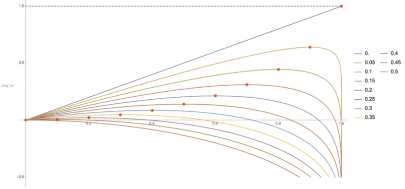
• Vertical axis is pay-off
• Horizontal axis is bet size
• Coloured curves show expected long-term pay-offs for a given bet-size for a given odd. Each coloured curve represents different odds. From top, blue line 0 is 0% chance of losing. From bottom, red curve is 50% chance of losing. 
• Red dot on coloured curve is optimal bet size (Kelly bet) that maximizes pay-off for a given odd in the long-run. 

Clearly, if your losing odd is 0%, the optimal bet size is 100%. Go all-in if you can’t lose. The more favourable the bias, the more aggressive you should be. Conversely, if your losing odds is more than 50%, the optimal bet size is 0% of your stack. 

Note that even if your odds of losing is just 5%, if you gamble too consistently, you’ll get caught in an unrecoverable losing spiral. This is shown to the right of the red dot on the chart.

There are two methods to consider in a risky strategy…

The first is to know all parameters about the future and engage in optimized portfolio construction, a lunacy unless one has a god-like knowledge of the future. …one needs to know the entire joint probability distribution of all assets for the entire future, plus the exact utility function for wealth at all future times. And without errors!

[Second], Kelly’s method… requires no joint distribution or utility function. It is very robust. …estimate the ratio of expected profit to worst- case return– dynamically adjusted to avoid ruin. …worst case is guaranteed (leave 80% or so of your money in reserves)… So, assuming one has the edge (as a sole central piece of information), engage in a dynamic strategy of variable betting, getting more conservative after losses (“cut your losses”) and more aggressive “with the house’s money”. 

The first strategy was only embraced by academic financial economists –empty suits without skin in the game — because you can make an academic career writing BS papers with method 1 much better than with method 2. On the other hand EVERY SURVIVING speculator uses explicitly or implicitly method 2 (evidence: Ray Dalio, Paul Tudor Jones, Renaissance, even Goldman Sachs!) For the first method, think of LTCM and the banking failure.

– Nassim Taleb’s Amazon book review of Kelly Capital Growth Investment Criterion

 

---

2. Ergodicity economics

While most financial systems are non-ergodic, the foundations of classical economic theory rests on fallacious ergodic assumptions. Equilibrium is not the natural state of the economy. Many models remove time from their equations by reducing it into an ensemble equivalent. This results in a false sense of security and optimism in most aggregate measurements, and risk management approaches. The importance of a quantity’s path through time is underestimated. 

 

2.1. Modern Portfolio Theory

Modern portfolio theory stipulates that there exists some optimal risk-to-return profile.

But the theory rests on the ergodic hypothesis by conflating an ensemble aggregate return with the individual’s path-dependent return through time. 

Modern Portfolio Theory utilizes ensemble or average returns to calculate a portfolio’s expected return. However, an individual portfolio manager is not interested in the ensemble return but in the individual portfolio’s return through time (i.e., the path-dependent return). The catch is that ensemble and time average returns are NOT equal because the distribution of returns is not normal. This is referred to as non-ergodic. – Complexity Investing whitepaper, NZS Capital

Read more about Modern Portfolio Theory as its pitfalls in my book notes on Misbehaviour of Markets by Mandelbrot.

 

2.2. DCF models

The DCF (discounted cash flow) model is the textbook method for valuing a company. Basically it involves summing all future cash flows while valuing future dollars that are further out from now as less than dollars today. This model assumes ergodicity because it reduces the time dimension by converting it into an ensemble expectation value – the net present value. While it’s useful in some instances, as with all models, we need to be well informed of its assumptions and limitations.

First, the discount factor applied is constant over time – an assumption that doesn’t hold up particularly well. Second, this constant discount rate typically comes from the weighted average cost of capital (WACC), which in turn is based on the contentious notion of equity risk premium and beta – both of which are easy to manipulate.

Quick detour on modern portfolio theory for those unfamiliar

• y = α + β+ ε 
• y, gamma = return of security
• α, alpha = idiosyncratic factors specific to this security
• β, beta = co-movement with relevant market indices
• ε, epsilon = everything else
• Equity risk premium is the additional risk on top of beta, that is, on top of the general market risk

All of these concepts in the DCF model derives from the Capital Asset Pricing Model, which derives from Expected Utility Theory, which derives from a 1738 Bernoulli paper, which had a critical math error that was only pointed out recently (by Ole Peters). Here’s the TED talk on it.

 

2.3. From GDP to DDP

GDP (gross domestic product): a measure popularized during the production era amidst and post-WWII to dimension get a quantitative grasp on economic activity, and a proxy for measuring national prosperity. Much of the criticisms center on what it excludes: environmental sustainability, its emphasis of having a trade surplus, social/cultural/emotional factors such as happiness, and other well-justified formula-imperfection-picking. Meanwhile, less often discussed is recognizing that GDP is an ensemble value. It assumes ergodicity. 

Remember, for something to be ergodic, what happens to the aggregate (ensemble-average) needs to be the same as what happens to the individual over time (time-average). When we say GDP increased by 2.3% and people applaud, that’s a reference to an aggregate increase of 2.3%. As we saw in the non-ergodic distribution in our rigged coin-flip game, this average outcome is far from a representative one for most individuals. Growth in GDP is a poor indicator for wealth growth at an individual level. Because a few really rich people pull up the average.

Ole Peters writes about a democratic domestic product (DDP). In a hypothetical country, 100 have an income of $50k/year. Suppose in the next year, one person enslaves everyone and steals all of their income ($5m = $50k x 100). The GDP would show as the same even though majority of people are now worse off. If this one person somehow grows his income from $5m to $5.5m, the country would show a 10% growth. Essentially, under this plutocratic system, GDP is weighted by the dollar, not by the individual. 

Alternatively, what if we computed the aggregate growth not as a dollar-weighted average growth (ensemble), but as a time-average for each of the individuals. That is, we take the income growth rate for each individual, and then average those averages. DDP gives equal weight to the individual rather than to the dollar. In this scenario, this DDP growth would show as a big fat negative number as majority of people saw reductions. 

 

---

3. Living in bets

So how am I practically applying ergodicity in everyday life?

In 3 ways.

 

3.1. Avoid doing really stupid shit

Our lives are non-ergodic. It’s path-dependent on time. Put simply, we only live once.

There’s 2 types of risks. One is recoverable, the other is not.

For an individual, unrecoverable risks include death, permanent disability, severe mental illness, unrecoverable personal brand damage (committing severe crime) etc.

So I take pretty standard measures to minimize these probabilities: take extra caution on the road, don’t get into fights etc.

Then there’s the less obvious but much more prevalent things that kill you slowly: excessive stress, poor quality sleep, bad nutrition etc. (Note: Cardiovascular disease is leading cause of death. Sleeping less than 6 hours a day increases risk of cardiovascular disease by 20%. Pareto-optimize health outcomes: focus on the 20% of actions that translate to 80% of the results. For both physical and mental health.)

Personally, I know I’m more exposed to unrecoverable risks from my travels. My obsession with under-rated destinations has taken me to places like: Mongolia, Siberian part of Russia, Myanmar, Uzbekistan, Kyrgyzstan, Ethiopia, and Uganda.

On trips like these I’ve run into all sorts of trouble. Encountering crocodiles while white-water rafting, confronting a thief who broke into room while I was asleep, driving a motorbike on winter mountain roads with frozen fingers, getting stranded in a desert for several hours amidst a violent tribal conflict, riding a horse at full speed without any training or proper equipment, and being in taxi speeding down a country highway at night with no working headlights.

My intention is not to glorify dangerous travel. I look back at such moments and classify them into one of 3:

• (i) “That was fun and I’d do it again.”
• (ii) “That was fun, but some things are only fun the first time.”
• (iii) “That was so fucking stupid. You could have died. Narrowly missed out on a Darwin Award. I’ll never put myself in that position again.”

So now, I’m more cautious and prepare more thoroughly for type (i) and (ii), and do all I can to reduce the probability of (iii) from occurring.  Pay more for safer transportation arrangements, secure accommodation, reliable tour operators etc.

“One may be risk loving yet completely averse to ruin… In a strategy that entails ruin, benefits never offset risks of ruin… Every single risk you take adds up to reduce your life expectancy… Rationality is avoidance of systemic ruin.” – Skin in the Game (2018), Nassim Taleb

I still want to visit some more wild/chaotic places, but I won’t take unnecessarily high risk of death just to ease my travel bug. Understanding ergodicity has shifted my pragmatism-adventure balance.

“…three distinct sides of risk:

• The odds you will get hit.

• The average consequences of getting hit.

• The tail-end consequences of getting hit.

…The first two are easy to grasp. It’s the third that’s hardest to learn, and can often only be learned through experience… Tail-end events are all that matter.” – The Three Sides of Risk, Collaborative Fund

 

3.2. Responding to luck: focus on what’s in control

Another implication of the ergodicity simulation we covered is luck.

To borrow from the modern portfolio theory equation again, I conceptualise life ‘success’ as something like this:

• y = f (α, β, ε) = a function of α, β, ε.
• y, gamma = ‘success’ in life. Can be defined in many ways.
• α, alpha = a pinch of genetic endowment, but mostly grit, growth-mindset, skills, experiences etc
• β, beta = your environment and your network
• ε, epsilon = luck, and other unexpected factors e.g. if world suddenly changes such that the niche skills you had suddenly becomes in hot-demand

As I learn more about how the world works, it seems that many conventionally success people continue to under-play the role of luck. Yes they all worked hard, but they all had luck on their side – in some shape or form.

We saw the magnitude of of absurd unequal distributions that a simple coin flip game can yield. Even in a world with favourable ensemble odds, you need a healthy amount of luck on your side to come out ahead (without applying Kelly criterion that is).

I’m not talking about net wealth, but rather a higher level dimension. If you want to be rich, why? Then why again? Then why again? Eventually you’ll hit an end-point. I ended up with something like fulfillment. Others might call it happiness. Doesn’t matter. Let’s not get pedantic with the semantics. That’s the highest level dimension that you’re optimising for. That’s the thing that I’m talking about now.

Now I’m not saying luck is the only path to ‘success’ in a defeatist manner. I’m saying that luck seems to have a bigger role than what I previously thought. I still value alpha (grit, growth mindset etc), but I’ve also incorporated the effect of Black Swans, luck, and ergodicity into my life model (epsilon). 

Based on this belief – the disproportionately high-value of luck – what do I do?

My answer: just focus on what’s in control. The alpha, and partially, beta.

If luck comes, great. If it doesn’t, all good. Either way, I’m fulfilled. I really did my best – what more could I ask for.

If it turns out that luck really can be controlled to some extent – work the subconscious, energy vibrations, law of attraction, hard work attracts luck etc – then great, I’ve got pretty good exposure to a lot of that stuff too. If not, all good. I’ve still derived a happiness utiility from the positive thoughts. It’s a set-up for large uncapped exposure with a capped downsize risk – a strategy I discussed in detail when articulating antifragility and optionality.

So for now, I’m confident living by the principle, focus on what’s in control. 

 

3.3. Make Kelly bets in major life decisions

Life is an accumulation of bets we’ve made (as well as bets made by our parents, and the society we grew up in etc). The future is also just a series of bets. A non-ergodic path-dependent sequence.

Some bets have higher stakes than others: changing jobs, re-locating, picking a lifelong partner etc. And other bets seem like lower stakes, but due to their frequency, accumulate into high stakes – e.g. lifestyle choices. Each bet is associated with a pay-off/return, potential loss/downside, and a probability. The currency of the downside, the thing we’re gambling, is typically our time.  

So it’s worth putting in more conscious effort into assessing the favourability of a bet. Especially for higher stakes. Let the beauty of asymmetry compound. Set yourself up so that time is more of an ally than an enemy. Sure, you could still go bust by getting hit by a bus tomorrow. But what can you do. Getting as close as possible to favourable bets and making lots of them is an optimal life strategy.

Extremely conceptual (even by my standards), but I ask myself: “Is there some Kelly criterion that’s applicable here to adjust the bet size to maximize the pay-off?” 

In practice, we don’t know the exact odds. Even if we did, it’ll change over time. It’s a Bayesian probability. We don’t know the pay-out. And even if we did, we wouldn’t have the computing power, or time to conduct thorough analysis. We’d be at the mercy of analysis paralysis.

But we can still try. Keep calibrating the guide in your head that tells you what’s worthwhile, and what’s important. That’s what really counts.

P.S. Did you notice the title of this post also makes an ergodic assumption? 😉

---

Found this useful? Can treat me to a coffee 🙂

Or simply share this post with your friends.

Drop your email below for a once-every-few-weeks newsletter packed with a curation of ideas that have kept me up at night.

---

If you enjoyed this, you may also like:

Antifragility, Modernity, and Dancing with Disorder

Common Knowledge: Consensus View of the Consensus View

Muffin or Chihuahua: Confusion Matrix and the Base Rate Fallacy